
Field-style article image prepared for centrifugal pump curves.
A centrifugal pump curve is a decision sheet, not just a performance graph. It shows whether the required duty point sits in a stable operating region, whether the pump is near its best efficiency range, and whether power and NPSH requirements fit the motor and suction conditions. Reading the curve correctly prevents a selection that works only at one narrow point.
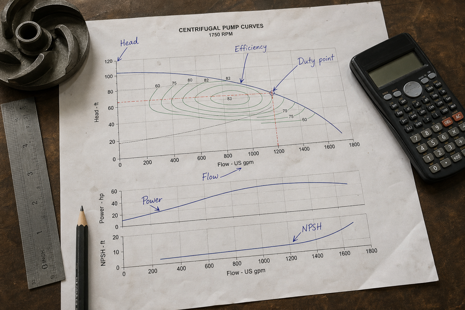
Centrifugal pump curves plot performance across the operating range. The head-flow curve shows how discharge pressure drops as flow increases. The efficiency curve identifies the zone where the pump converts shaft power to hydraulic work most effectively. The brake horsepower curve shows input power demand at each flow rate. Together, these curves let you confirm the pump will meet system requirements, operate efficiently, and stay within driver capacity.
Key Takeaways
- The head-flow curve shows the inverse relationship between discharge head and flow rate at constant speed.
- Peak efficiency typically occurs at 60-80% of the pump’s maximum flow, defining the preferred operating range.
- The system curve intersects the pump curve at the operating point, which determines actual head and flow in the installed system.
- Operating far from best efficiency point increases energy cost, vibration, and seal or bearing wear.
- Brake horsepower rises with flow; the motor must handle maximum power across the anticipated operating range.
Reading the Head-Flow Curve
The head-flow curve traces total dynamic head against volumetric flow at a fixed impeller diameter and rotational speed. Head decreases as flow increases because larger flow rates create higher internal losses in the impeller and volute. A steep curve shows head dropping rapidly with flow. A flat curve maintains head across a wider flow range.
Steep curves suit applications with variable system resistance, such as batch filling or level control. Small flow changes produce large head swings that help throttle valves or VFDs regulate precisely. Flat curves suit constant-pressure applications where parallel pumps share load, because head remains stable as individual pump flows vary.
The shutoff head at zero flow and the maximum flow at zero head define the curve envelope. Most pumps should not operate continuously near either extreme. Shutoff operation traps energy in the casing, overheating the fluid and stressing seals. Running out on the curve toward maximum flow risks cavitation, recirculation, and radial thrust on the shaft.
Locating the Efficiency Island
The efficiency curve usually appears as concentric contour lines or a single peak line overlaid on the head-flow plot. Peak efficiency—often called best efficiency point or BEP—typically occurs at 60 to 80 percent of maximum flow. Operating within 70 to 110 percent of BEP flow keeps efficiency high and mechanical stress low.
Efficiency drops at low flow due to recirculation and slip losses. At high flow, friction and turbulence losses increase. The efficiency island shows where acceptable efficiency holds, often bounded by contours at 2-3 points below peak. Selecting a pump so the required duty point falls inside this island ensures low energy cost and long component life.
For a 100-hp pump running 8,000 hours per year at $0.10/kWh, a 5-point efficiency drop costs roughly $3,000 annually in extra energy. Specifying the wrong pump or operating far off BEP compounds over the asset life. High-specific-speed pumps (axial-flow types) show flatter, broader efficiency curves. Low-specific-speed pumps (high-head, low-flow types) have steeper curves with narrower efficient ranges.
Understanding Brake Horsepower Requirements
The brake horsepower (BHP) curve shows input power to the pump shaft across the flow range. Power generally increases with flow because both head and flow contribute to hydraulic power (P = ρ × g × Q × H / η). Even though head drops at higher flow, the product often rises, demanding more shaft power.
Non-overloading curves show power peaking before maximum flow, then declining. Overloading curves show power rising continuously to maximum flow. With an overloading curve, the motor must handle full-flow power even if the normal duty point is lower. Undersizing the motor on an overloading pump causes nuisance trips when the system resistance drops or a valve opens.
The motor nameplate horsepower must exceed the maximum BHP anywhere in the expected operating range, including transient conditions. A service factor of 1.15 allows a 100-hp motor to deliver 115 hp briefly, providing margin for startup, fouling, or off-design operation.
Plotting the System Curve and Operating Point
The system curve plots total head required against flow rate for the piping network. Static head (elevation change, tank pressure) is constant across all flows. Friction head follows the square law: doubling flow quadruples friction losses. The system curve equation takes the form H_sys = H_static + K × Q².
The operating point occurs where the pump curve intersects the system curve. At this intersection, the pump delivers exactly the head needed to overcome system resistance at the resulting flow. If the system curve shifts right (lower resistance), flow increases and head drops along the pump curve. If resistance increases, the operating point moves left toward higher head and lower flow.
Mismatches between predicted and actual system curves cause off-design operation. Fouled heat exchangers, partially closed valves, or incorrect pipe roughness estimates shift the system curve. Always plot the system curve from the same datum as the pump curve—usually pump centerline or suction flange—to avoid elevation errors.
Worked Example: Verifying a Duty Point
A cooling water pump must deliver 1,200 gpm against a system with 40 feet of static head and an estimated friction coefficient K = 0.00015 ft/(gpm)². At 1,200 gpm, friction head = 0.00015 × 1,200² = 216 feet. Total system head = 40 + 216 = 256 feet.
The proposed pump curve shows 260 feet at 1,200 gpm, 75% efficiency, and 110 BHP. The system requires 256 feet; the pump provides 260 feet. The slight excess means the pump will deliver approximately 1,220 gpm (where the pump curve intersects 256 feet), assuming the system curve calculation is accurate.
At 1,200 gpm, the pump’s BEP is listed at 1,100 gpm. Operating at 1,200 gpm is 109% of BEP flow—acceptable within the 70-110% guideline. Efficiency at 75% is 2 points below peak (77%), so energy penalty is minimal. The 110 BHP requires a 125-hp motor with service factor, or a 150-hp motor for margin on an overloading curve.
If the actual system friction is higher than estimated—K = 0.00020 instead of 0.00015—the friction head at 1,200 gpm becomes 288 feet, and total system head is 328 feet. The operating point would shift left along the pump curve, reducing flow to perhaps 1,050 gpm. Confirming friction estimates through pressure-drop calculations or flow tests prevents this undercapacity scenario.
Adjusting Performance with Speed and Impeller Trim
Affinity laws describe how pump performance scales with speed or impeller diameter changes. Flow varies directly with speed (Q₂/Q₁ = N₂/N₁). Head varies with speed squared (H₂/H₁ = (N₂/N₁)²). Power varies with speed cubed (P₂/P₁ = (N₂/N₁)³).
Reducing speed by 20% cuts flow by 20%, head by 36%, and power by 49%. Variable frequency drives exploit this relationship to match pump output to system demand while saving energy. Slowing the pump moves the entire curve downward and left; the operating point shifts along the system curve.
Impeller trimming reduces impeller diameter to lower the curve permanently. Trim curves are often shown as dashed lines on the pump curve sheet. A 10% diameter reduction typically lowers head by 19% and flow by 10% at constant speed. Trimming avoids throttling losses when the pump is oversized, but it cannot be reversed without replacing the impeller.
FAQs
What does a drooping head-flow curve indicate?
A sharply drooping curve means the pump develops significantly less head at higher flows. This shape is common in low-specific-speed radial-flow pumps. It provides good flow regulation with throttle control but limits the maximum flow range. Drooping curves also mean parallel pumps may not share load evenly unless system resistance is carefully balanced.
Can I use a pump curve generated at different fluid properties?
Pump curves are usually published for clear water at 68°F. Viscosity, density, and vapor pressure affect performance. High-viscosity fluids reduce flow, head, and efficiency due to increased friction. The Hydraulic Institute provides correction factors for viscous liquids. Pumping hot water or light hydrocarbons requires NPSH adjustments to avoid cavitation, but the head-flow shape remains valid if corrected for density.
Why do some pumps show multiple curves on one chart?
Multiple curves typically represent different impeller diameters within the same casing. A size 4×6-13 pump might show curves for 12-inch, 12.5-inch, and 13-inch impellers. This lets you select the diameter that places your duty point closest to BEP without changing the pump frame. Some charts also overlay curves for different speeds, especially for belt-driven or VFD-controlled pumps.
How do I account for wear or fouling over time?
Pump curves represent new, clean conditions. Impeller wear, casing ring clearance growth, and surface roughness from corrosion or scaling reduce head by 2-10% over several years. Specifying the pump so the duty point starts slightly left of BEP provides margin for degradation. Schedule predictive maintenance based on performance testing against the original curve to catch wear before efficiency falls sharply.
Conclusion
Reading centrifugal pump curves correctly requires plotting the system curve and confirming the intersection falls within the efficiency island. Verify that brake horsepower stays within motor capacity across the full operating range, including transient or fouled conditions. When the duty point sits near the curve edges or outside the efficiency contours, request a different impeller diameter or consider a different pump frame. Accurate curve interpretation during selection prevents costly retrofits, high energy bills, and premature failures once the pump is installed.